\[ f(x_i)\geq 0\qquad\forall x_i \] \[ \sum_{i=1}^n f(x_i)=1 \] \[ F(x_i)=P(x_j\leq x_i)=\sum_{x_j\leq x_i}f(x_j) \] \[ \expected{g(X)}=\sum_{i=1}^n g(x_i) f(x_i) \]

$f(x_i)$ is the probability distribution function (PDF) and $F(x_i)$ is the cumulative distribution function (CDF). $\expected{g(X)}$ is the expected value of $g(X)$.

Edit

8.2 Continuous probability distribution

\[ f(x)\geq 0\qquad\forall x \] \[ \int_{-\infty}^{+\infty}f(x)\,dx=1 \] \[ F(x)=P(x’\leq x)=\int_{-\infty}^x f(x’)\,dx’ \] \[ \expected{g(X)}=\int_{-\infty}^{+\infty}g(x) f(x)\,dx \]

Edit

9 Important statistics

$\mu_x$: Arithmetic average or mean of $X$ if $g(x)=x$; measure of the average

$\sigma_x^2$: Variance of $X$ if $g(x)=(x-\mu_x)^2$; measure of the variability about the average

$g_x$: Skewness of $X$ if $g(x)=\frac{(x-\mu_x)^3}{\sigma_x^3}$; measure of the symmetry about the average

Edit

9.1 Example 5.1 (Chin 2000)

A water-resource system if designed such that the probability, $f(x_i)$, that the system capacity is exceeded $x_i$ times during the 50-year design life is given by the discrete probability distribution in the table. What is the mean number of system failures expected in 50 years? What is the variance and skewness of the number of failures?

$\mu_x=2$
$\sigma_x^2=1.92$
$g_x=0.631$

$x_i$	$f(x_i)$
0	0.13
1	0.27
2	0.28
3	0.18
4	0.09
5	0.03
6	0.02
>6	0.00

Edit

9.2 Homework: Example 5.2 (Chin 2000)

The probability density function, $f(t)$, of the time between storms during the summer in Miami is estimated as \[ f(t)=\begin{cases} 0.014 e^{-0.014t}& t>0\\ 0& \text{otherwise} \end{cases} \] where $t$ is the time interval between storms in hours. Estimate the mean, standard deviation, and skewness of $t$.

Use these facts: \[ \int_0^\infty e^{-ax}\,dx=\frac{1}{a},\qquad \int_0^\infty x e^{-ax}\,dx=\frac{1}{a^2},\qquad \int_0^\infty x^2 e^{-ax}\,dx=\frac{2}{a^3},\qquad \int_0^\infty x^3 e^{-ax}\,dx=\frac{6}{a^4} \]

$\mu_t=71 \text{h}$
$\sigma_t=71 \text{h}$
$g_t=2.1$

Edit

10 Normal distribution

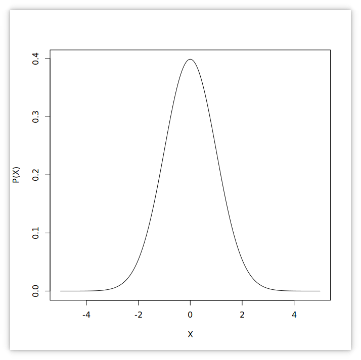
Statisticians and probabilists love normal distributions thanks to the central limit theorem.

\[f(x)=\frac{1}{\sigma\sqrt{2\pi}}e^{-\frac{1}{2}\left(\frac{x-\mu}{\sigma}\right)^2}\] where

$x$ is a random variable,
$\mu$ is the mean or expected value of $x$, and
$\sigma$ is the standard deviation.

Standard normal distribution when $\mu=0$ and $\sigma=1$.

Edit

11 Central limit theorem

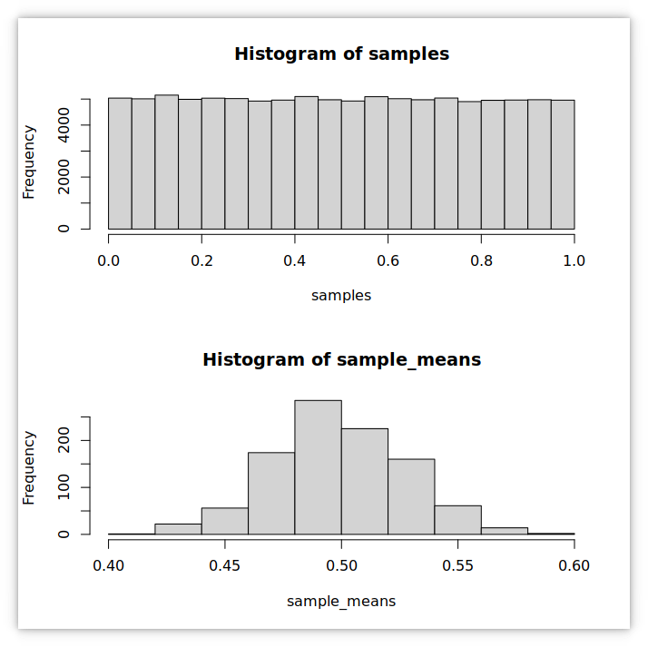
# R code by Huidae Cho
samples <- c()
sample_means <- c()
for(i in 1:1000){
  sample <- runif(100)                          # take 100 random values from a uniform distribution
  samples <- c(samples, sample)                 # collect samples
  sample_means <- c(sample_means, mean(sample)) # collect sample means
}
par(mfcol=c(2,1))
hist(samples)                                   # plot the histogram of samples
hist(sample_means)                              # plot the histogram of sample means

Edit

12 Hypothesis testing

Hypothesis testing is a quantitative inferential statistical method to see whether your data statistically supports a certain hypothesis.

Edit

12.1 Null hypothesis

A default position that there is no significant relationship between two phenomena or among groups.

Often, denoted by $H_0$.

We never accept the null hypothesis. We only reject or fail to reject it given the level of confidence ($\alpha$-level).

Edit

12.2 Alternative hypothesis

A hypothesis that there is significant relationship between two phenomena or among groups.

Denoted by $H_a$.

Edit

12.3 What is the $\alpha$-level?

The $\alpha$-level or significance level indicates how extreme observed data must be before we can reject the null hypothesis.

Edit

12.4 A $p$-value?

The $p$-value is the probability that we observe a certain phenomenon under the null hypothesis.

Edit

12.5 Testing hypotheses

If the $p$-value is less than or equal to the $\alpha$-level, our data is unusual—more extreme than the significance level—and we reject the null hypothesis. We can say the data is statistically significant with a significance level of $\alpha$. In this case, the alternative hypothesis is supported, not accepted.

If the $p$-value is greater than the $\alpha$-level, the data is usual—not as extreme as the significance level—and we fail to reject the null hypothesis. We can say the data is statistically non-significant with a significance level of $\alpha$.

Edit

12.6 Exercises

Edit

12.7 Chi-squared test

A $\chi^2$ test is a statistical method to test if data follows a certain probability distribution.

If $N$ observations are divided into $M$ classes and $X_m$ indicates the number of observations in class $m$, the following random variable \[ \chi^2=\sum_{m=1}^M\frac{(X_m-Np_m)^2}{Np_m} \] follows a chi-square distribution where $p_m$ is the theoretical probability of an observation in class $m$.

The number of degrees of freedom is $M-1-n$ where $n$ is the number of population parameters estimated using sample statistics.

We fail to reject the null hypothesis that samples are drawn from a certain probability distribution if $0\leq\chi^2\leq\chi_\alpha^2$.

Edit

12.8 Example 5.16 (Chin 2000)

Analysis of a 47-year record of annual rainfall indicates the following frequency distribution:

Range (mm)	Number of outcomes	Range (mm)	Number of outcomes
<1,000	2	1,250–1,300	7
1,000–1,050	3	1,300–1,350	5
1,050–1,100	4	1,350–1,400	3
1,100–1,150	5	1,400–1,450	2
1,150–1,200	6	1,450–1,500	2
1,200–1,250	7	>1,500	1

The measured data also indicate a mean of 1,225 mm and a standard deviation of 151 mm. Using a 5% significance level, assess the hypothesis that the annual rainfall is drawn from a normal distribution.

Use these tables:

Edit

13 Homework: Problem 5.1 (Chin 2000)

A flood-control system is designed such that the probability that the system capacity is exceeded $X$ times in 30 years is given by the discrete probability distribution in the table.

What is the mean number of system failures expected in 30 years? What is the variance and skewness of the number of failures?

$x_i$	$f(x_i)$
0	0.04
1	0.14
2	0.23
3	0.24
4	0.18
5	0.10
6	0.05
7	0.02
8	0.01
>9	0.00

Edit

14 Reading materials

Edit