Pipelines
Department of Civil and Environmental Engineering...New Mexico State University
Contents
- 1 What is pipe flow?
- 2 Energy equation for pipe flow
- 3 Head loss model
- 4 Reynolds number
- 5 Example 1: Laminar flow
- 6 Friction factor in turbulent flow
- 7 Moody diagram
- 8 Example 2: Turbulent flow
- 9 Single pipe workflow
- 10 Colebrook equation practice
- 11 Minor losses practice
- 12 Homework: Pipelines
- 13 Pipe networks preview
1 What is pipe flow?
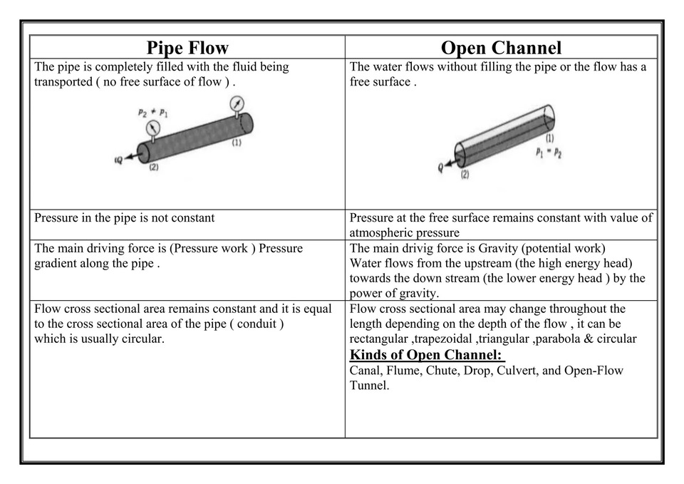
- No free surface (flow full)
- Driven by pressure head difference
- Analyzed using Darcy–Weisbach equation
1.1 Key distinction: Open channel vs pipe flow
| Open channel flow | Pipe flow |
|---|---|
| Free surface | No free surface |
| Driven by slope | Driven by pressure difference |
| Manning equation | Darcy–Weisbach equation |
2 Energy equation for pipe flow
General energy equation:
\[ \frac{P_1}{\gamma} + \frac{V_1^2}{2g} + z_1 - h_L = \frac{P_2}{\gamma} + \frac{V_2^2}{2g} + z_2 \]For constant diameter pipes ($V_1 = V_2$):
\[ h_L = \left(\frac{P_1}{\gamma} + z_1 \right) - \left(\frac{P_2}{\gamma} + z_2 \right) \]Key points:
- $h_L$ represents energy dissipation.
- Hydraulic grade line (HGL): $P/\gamma + z$
- Energy grade line (EGL): $P/\gamma + z + V^2/(2g)$
3 Head loss model
Major loss (friction):
\[ h_f = f \frac{L}{D} \frac{V^2}{2g} \]Minor loss:
\[ h_m = K \frac{V^2}{2g} \]Total head loss:
\[ h_L = h_f + \sum h_m \]4 Reynolds number
\[ Re = \frac{VD}{\nu} \]Flow regimes:
- Laminar: $Re < 2000$
- Transitional: $2000 \le Re \le 4000$
- Turbulent: $Re > 4000$
Question:
- What physical forces compete in $Re$?
5 Example 1: Laminar flow
Given:
- $\nu = 2.0 \times 10^{-4} \ \text{m}^2/\text{s}$
- $D = 0.05 \ \text{m}$
- $L = 20 \ \text{m}$
- $Q = 1.0 \times 10^{-4} \ \text{m}^3/\text{s}$
- Compute velocity:\[ V = \frac{Q}{\pi D^2/4} \]
- Compute Reynolds number:\[ Re = \frac{VD}{\nu} \]
- Determine regime
- If laminar, compute friction factor:\[ f = \frac{64}{Re} \]
- Compute head loss:\[ h_f = f \frac{L}{D} \frac{V^2}{2g} \]
Key points:
- No roughness required.
- Fully analytical solution.
6 Friction factor in turbulent flow
Colebrook equation:
\[ \frac{1}{\sqrt{f}} = -2 \log_{10} \left( \frac{\varepsilon}{3.7D} + \frac{2.51}{Re\sqrt{f}} \right) \]Key points:
- $f$ depends on $Re$.
- $f$ depends on relative roughness $\varepsilon/D$.
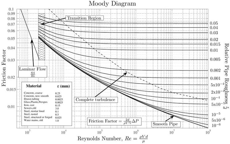
7 Moody diagram
Inputs:
- Reynolds number
- Relative roughness $\varepsilon/D$
Output:
- Friction factor $f$
Important regions:
- Laminar region
- Smooth pipe limit
- Fully rough region
8 Example 2: Turbulent flow
Given:
- $\nu = 1.0 \times 10^{-6} \ \text{m}^2/\text{s}$
- $D = 0.20 \ \text{m}$
- $L = 300 \ \text{m}$
- $Q = 0.05 \ \text{m}^3/\text{s}$
- $\varepsilon = 0.046 \ \text{mm}$
- Compute velocity:\[ V = \frac{Q}{\pi D^2/4} \]
- Compute Reynolds number:\[ Re = \frac{VD}{\nu} \]
- Compute relative roughness:\[ \frac{\varepsilon}{D} \]
- Read friction factor from Moody diagram
- Compute head loss:\[ h_f = f \frac{L}{D} \frac{V^2}{2g} \]
Key points:
- Roughness matters in turbulent flow.
- Follow the algorithm step by step.
9 Single pipe workflow
Remember:
- Compute velocity:\[ V = \frac{Q}{A} \]
- Compute Reynolds number:\[ Re = \frac{VD}{\nu} \]
- Determine regime
- Obtain friction factor $f$
- Compute head loss:\[ h_f = f \frac{L}{D} \frac{V^2}{2g} \]
If you remember this sequence, you can solve any single-pipe problem.
10 Colebrook equation practice
10.1 Problem 1: Friction factor from Colebrook (given $Re$ and $\varepsilon/D$)
Given:
- $Re = 2.0 \times 10^5$
- $\varepsilon/D = 2.0 \times 10^{-4}$
Tasks:
- Solve the Colebrook equation for $f$.
- Report $f$ to three significant digits.
- State whether the pipe is closer to the smooth limit or fully rough limit.
Colebrook equation:
\[ \frac{1}{\sqrt{f}} = -2 \log_{10} \left( \frac{\varepsilon}{3.7D} + \frac{2.51}{Re\sqrt{f}} \right) \]10.2 Problem 2: Friction factor from Colebrook (higher roughness)
Given:
- $Re = 8.0 \times 10^5$
- $\varepsilon/D = 3.0 \times 10^{-3}$
Tasks:
- Solve for $f$ using the Colebrook equation.
- Compare your result to the fully rough approximation (optional discussion).
10.3 Problem 3: Friction factor sensitivity to Reynolds number
Given:
- $\varepsilon/D = 5.0 \times 10^{-4}$
- Case A: $Re = 5.0 \times 10^4$
- Case B: $Re = 5.0 \times 10^6$
Tasks:
- Solve for $f$ for Case A and Case B.
- Explain why $f$ changes (or does not change much) as $Re$ increases.
10.4 Problem 4: Determine $Re$ required to reach a target friction factor
Given:
- $\varepsilon/D = 1.0 \times 10^{-4}$
- Target: $f = 0.020$
Tasks:
- Solve the Colebrook equation for $Re$.
- State whether the required $Re$ is realistic for typical water distribution systems ($V$ within 0.5 to 2 m/s, sometimes up to 3 m/s, but rarely beyond that).
11 Minor losses practice
11.1 Problem 5: Total minor loss coefficient and head loss
Given:
- Water at 20°C
- $D = 0.10 \ \text{m}$
- $Q = 0.012 \ \text{m}^3/\text{s}$
- Minor loss coefficients:
- Entrance (sharp): $K = 0.50$
- Two standard 90° elbows: $K = 0.90$ each
- Gate valve (fully open): $K = 0.15$
- Exit: $K = 1.00$
Tasks:
- Compute $V$.
- Compute total $K$.
- Compute minor head loss $h_m$.
Minor loss equation:
\[ h_m = K \frac{V^2}{2g} \]11.2 Problem 6: Minor vs major loss comparison
Given:
- Water at 20°C
- $D = 0.08 \ \text{m}$
- $L = 40 \ \text{m}$
- $Q = 0.006 \ \text{m}^3/\text{s}$
- $f = 0.022$
- Fittings:
- Four 90° elbows: $K = 0.90$ each
- One globe valve (fully open): $K = 10.0$
- Exit: $K = 1.0$
Tasks:
- Compute $V$.
- Compute major loss $h_f$.
- Compute minor loss $\sum h_m$.
- Compute percent of total head loss coming from minor losses.
Major loss equation:
\[ h_f = f \frac{L}{D} \frac{V^2}{2g} \]11.3 Problem 7: Solve for flow rate given available head (minor losses only)
Given:
- Water at 20°C
- $D = 0.05 \ \text{m}$
- Available head loss: $h_m = 3.0 \ \text{m}$
- Fittings:
- Entrance: $K = 0.50$
- Three 90° elbows: $K = 0.90$ each
- Ball valve (fully open): $K = 0.05$
- Exit: $K = 1.00$
Tasks:
- Compute total $K$.
- Solve for velocity $V$.
- Compute discharge $Q$.
11.4 Problem 8: Combined major and minor losses (design check)
Given:
- Water at 20°C
- $D = 0.15 \ \text{m}$
- $L = 250 \ \text{m}$
- $Q = 0.030 \ \text{m}^3/\text{s}$
- $f = 0.020$
- Fittings:
- Entrance: $K = 0.50$
- Two 45° bends: $K = 0.35$ each
- Butterfly valve (fully open): $K = 0.20$
- Exit: $K = 1.00$
Tasks:
- Compute $V$.
- Compute $h_f$.
- Compute $h_m$.
- Compute total head loss $h_L$.
Total head loss:
\[ h_L = h_f + \sum h_m \]11.5 Problem 9: Iterate because $f$ depends on $Re$
Given:
- Water at 20°C, $\nu = 1.0 \times 10^{-6} \ \text{m}^2/\text{s}$
- $D = 0.10 \ \text{m}$
- $L = 120 \ \text{m}$
- $\varepsilon = 0.046 \ \text{mm}$
- Available head loss: $h_L = 8.0 \ \text{m}$
- Fittings:
- Entrance: $K = 0.50$
- Four 90° elbows: $K = 0.90$ each
- Exit: $K = 1.00$
Tasks:
- Set up the equation for $h_L = h_f + \sum h_m$.
- Iterate to find $Q$ (or $V$) using Colebrook for $f$.
- Report final $Q$ and $f$.
Key points:
- This problem requires iteration because $f$ depends on $Re$ and $Re$ depends on $V$.
12 Homework: Pipelines
13 Pipe networks preview
Series condition:
\[ h_L = \sum h_{L,i} \]Parallel conditions:
\[ Q_T = Q_1 + Q_2 \] \[ h_{f,1} = h_{f,2} \]Next class:
- We solve network systems.

