Introduction to statistical hydrology
1 Statistics vs. probability
In summary, probability theory enables us to find the consequences of a given ideal world, while statistical theory enables us to measure the extent to which our world is ideal. Steve Skiena
1.1 Dice questions
- What is the probability of a die rolling a 1?
- What about a 1 and then a 6 in a sequence?
- A 1 and a 6 from two dice simultaneously?
2 Uncertainty
It all comes down to uncertainty!
We have to embrace uncertainty when studying science because we only have limited knowledge.
The lack of certainty or confidence is called uncertainty.
2.1 Epistemic vs. aleatory uncertainty
Epistemic uncertainty arises because of the lack of our knowledge.
Aleatory uncertainty arises because of randomness.
2.2 Sources of uncertainty
Morgan and Henrion (1990)
- random and/or systematic errors in measurements of a quantity
- linguistic imprecision derived from qualitative reasoning
- quantity variability over time and space
- inherent randomness
- unpredictability (chaotic behavior) of dynamical systems
- disagreement or different opinions among experts about a particular quantity
- approximation uncertainty arising from a simplified model of the real-world system
3 Inductive vs. deductive reasoning
Inductive reasoning starts with observations and analyzes data to formulate a theory.
Deductive reasoning starts with ideas or premises and observes data to make a conclusion.
4 Variables
What is a variable (often referred to as a random variable) in statistics and probability? A value that can vary!
Any characteristic of an object or event of interest that we can
- measure,
- record, and
- analyze.
5 Statistics in hydrology
- Hydrologic processes and variables
- Time series analysis
- Exceedance probability
- Return period
- Flood frequency analysis
- USGS regional regression equations
6 Hydrologic processes
Hydrologic processes relate flows of water to their occurrences in space and time, and they are formulated as models. Because of this simplification, there is uncertainty in space and time as a form of spatial and temporal variability.
Models can be
- Deterministic or
- Stochastic
7 Hydrologic variables
Hydrologic variables include
- Runoff discharge
- Evaporation rate
- Infiltration rate
- Streamflow
- Groundwater flow
- Rainfall
- Snowfall
Monitoring of these variables is typically done at discrete spaces and times.
8 Exceedance probability
The probability that a certain event will be exceeded.
8.1 Weibull plotting position
Commonly used for plotting hydrologic data.
\[P(X>x_m)=\frac{m}{N+1}\] where $N$ is the number of observations and $m$ is the rank from 1 for the largest to $N$ for the smallest.
Asymptotically exact only for a population from a uniform distribution (relatively rare in nature).
8.2 Gringorten plotting position
Addresses the shortcoming of the Weibull formula.
\[P(X>x_m)=\frac{m-a}{N+1-2a}\]
where $a=0.40$ is recommended for hydrology.
8.3 Example 5.15 (Chin 2000)
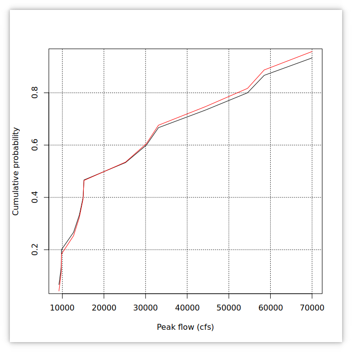
The annual peak flows in the Guadalupe River near Victoria, Texas, between 1965 and 1978 are shown in the table. Use the Weibull and Gringorten formulae to estimate the cumulative probability distribution of annual peak flow and compare the results.
| Year | Peak flow ($\text{ft}^3/\text{s}$) |
|---|---|
| 1965 | 15,000 |
| 1966 | 9,790 |
| 1967 | 70,000 |
| 1968 | 44,300 |
| 1969 | 15,200 |
| 1970 | 9,190 |
| 1971 | 9,740 |
| 1972 | 58,500 |
| 1973 | 33,100 |
| 1974 | 25,200 |
| 1975 | 30,200 |
| 1976 | 14,100 |
| 1977 | 54,500 |
| 1978 | 12,700 |
8.3.1 Example 5.15 solution
Q <- c(15000, 9790, 70000, 44300, 15200, 9190, 9740, 58500, 33100, 25200, 30200, 14100, 54500, 12700)
ord <- order(Q)      # order of peak flows for plotting
N <- length(Q)       # number of peak flows
m <- N - rank(Q) + 1 # 1 for largest
a <- 0.4
Weibull <- m / (N + 1)
Gringorten <- (m - a) / (N + 1 - 2 * a)
plot(Q[ord], 1 - Weibull[ord], type="l", xlab="Peak flow (cfs)", ylab="Cumulative probability")
grid(col="black")
lines(Q[ord], 1 - Gringorten[ord], col="red")9 Return period
Also referred to as the recurrence interval.
\[T=\frac{1}{P}\] where $P$ is the exceedance probability.
What does it mean? Does a 100-year flood ($T=100$ or $P=0.01$) occur only once in 100 years? A die example?
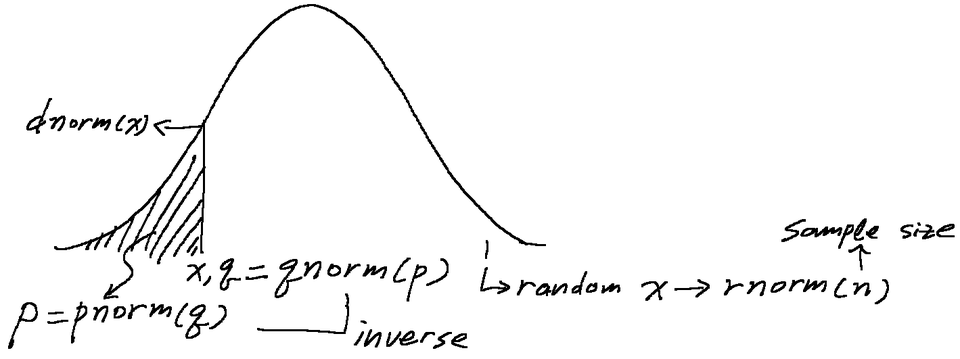
10 R probability functions
11 Reading materials
12 References
- Morgan, M. G., Henrion, M., 1990. Uncertainty—A guide to dealing with uncertainty in quantitative risk and policy analysis. Cambridge University Press, Cambridge.

